16 Apr 2020 - Harikrishnan N B
Aim of Physics
The aim of physics is to find the rules or uncover the mathematical equations that govern our universe. The second aim is to explain the observations. In order to explain the observations, we need to have multiple competing theories, models or hypothesis. The theory or the model should also predict the observations. We shall see some of these models.
Newton’s Model of Universe
Newton truly believed that the universe has the exact predictability of a machine. Everything has a order and deterministic nature. This boils down to writing differential equations. \(F = ma = m\frac{dv}{dt}\) If we know the position and momentum of all the particles in the universe and if a differential equation could be wrote then we could predict the infinite future using a computer. This is illustrated in the clockwork in Figure 1. Everything is quarks in the huge clock in Figure 1, it has an order and deterministic rules to predict the future. This was Newton’s model.
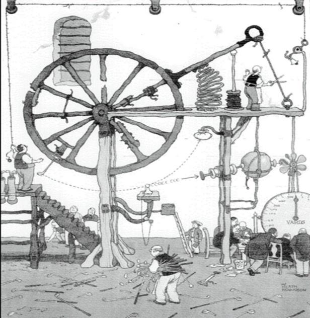
Figure 1: Newton’s Model of Universe (Image Source: https://www.wired.co.uk/gallery/heath-robinson-deserves-a-museum-gallery)
Laplace (1749-1827)
“An intelligence knowing, at a given instant of time, all forces acting in nature, as well as the momentary positions of all things of which the universe consists, would be able to comprehend the motions of the largest bodies of the world and those of the smallest atoms in one single formula, provided it were sufficiently powerful to subject all data to analysis. To it, nothing would be uncertain; both future and past would be present before its eyes.”
Laplace also believed in determinism.
Types of Systems
Deterministic: We know the rules, the initial positions and we can compute the future of all time. There is no randomness.
Quantum: We know that we can’t know the values beyond a certain limit (Heisenberg). For example, in Figure 2, we want to measure the position and velocity of electron. To do that we have to bombard photon’s of some energy to it. The act of measurement (bombardment), will change the direction of electron. In this scenario, to know something is to change or manipulate it.
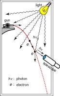
Figure 2: Quantum model (Image Source: https://www.physicsoftheuniverse.com/dates.html )
Gödel’s: These are formal axiomatic systems. In these systems there are statements which are true but cannot be proved true. So, there is a limit to know some truths at all.
Chaotic system has elements of all these three systems.
Is our Solar System Stable?
How are we sure that the orbits of all heavenly bodies are stable? or How do we know whether our moon will not fly away from its orbit tomorrow?
Sir Isaac Newton solved the two body problem. The moment when you have three bodies, then it turns out to be unsolvable.
Henri Poincaré showed that the problem is unsolvable because we cannot know the initial condition with infinite precision. Small perturbations in initial condition can give rise to different outcomes. So even if the universe is deterministic, it is unpredictable.
Chaos = Determinism + Unpredictability
Butterfly Effect - The tiny errors in the models, will lead to very different predictions. The flapping of the wings of a butterfly (equivalent to tiny errors in the model) can lead to different predictions (when compared to no flapping).
Because of this reason weather is impossible to predict for more than couple of weeks.
Chaos in Excel
Case I
-
Step 1: Take a number $0.2$.
-
Step 2: Multiply by $16$ and subtract $3$ =>$ 0.2* 16 - 3 = 3.2-3 = 0.2$.
-
Step 3: Now keep dragging. See what you observe?
We expect it will remain $0.2$. But it is not. Why?
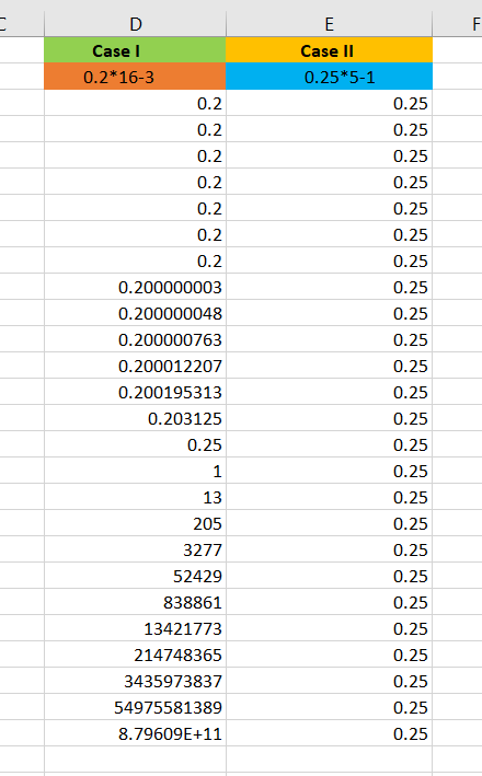
Figure 3: Chaos in Excel.
Case I in Figure 3 represents the dragging of $0.2 *16 - 3$. The binary expansion of $0.2$ has infinite precision. The binary expansion of $0.2$ is $0.\overline{0011}$. There is a truncation happening in the binary expansion of $0.2$ while computing each step. This truncation (tiny error) leads to very different prediction. At every step, we observe a truncation which leads to non-linearity and an iteration. Non-linearity and iteration are two important properties of chaos.
Case II
Now consider the following experiment in excel:
-
Step 1: Take a number $0.25$.
-
Step 2: Multiply by $5$ and subtract $1$ =>$ 0.25* 5 - 1 = 1.25-1 = 0.25$.
-
Step 3: Now keep dragging. See what you observe?
In this case, we do not notice any explosion as we found in Case I. This is because the binary expansion of $0.25$ is $0.01$, which is finite. Hence, there is no truncation happening (no nonlinearity) at each step. Case II is just a linear operation.
Henri Poincaré
“A very small cause which escapes our notice determines a considerable effect that we cannot fail to see, and then we say that the effect is due to chance. If we knew exactly the laws of nature and the situation of the universe at the initial moment, we could predict exactly the situation of the same universe at a succeeding moment. But even if it were the case that the natural laws had no longer any secret for us, we could still know the situation approximately. If that enabled us to predict the succeeding situation with the same approximation, that is all we require, and we should say that the phenomenon had been predicted, that it is governed by the laws. But is not always so; it may happen that small differences in the initial conditions produce very great ones in the final phenomena. A small error in the former will produce an enormous error in the latter. Prediction becomes impossible…”. (Poincaré)
Conditions for CHAOS
- Deterministic Equations
- Iterations
- Non-linearity
- Infinity of periodic orbits (dense)
- Infinity of non-periodic orbits
- Transitive orbit (mixing)
- Butterfly effect
Can we reduce the above list? Robert Devaney one of the chaos theorists has come up with three conditions which are necessary and sufficient.
Devaney’s Condition
Definition: A dynamical system $F$ is chaotic if:
- Periodic points of $F$ are dense.
- $F$ is transitive.
- $F$ depends sensitively on initial conditions.
In plain English, we can map the above three into the following:
- Elements of Regularity (periodicity implies regularity).
- Indecomposability ( A chaotic system cannot be broken down into smaller subsystems which are non interacting).
- Deterministic Unpredictability (sensitive dependence on initial conditions).
Mathematical notations
\[x_{n+1} = f(x_n)\]$x_n$ is the state variable (for eg. population at the $n$ -th instant of time).
The orbit/ trajectory of $x_0$ under the map $f$ is defined as follows: \(x_0 \rightarrow x_1 \rightarrow x_2 \rightarrow \ldots \rightarrow x_n \ldots\) This can also be written as : \(x_0 \rightarrow f(x_0) \rightarrow f^{2}(x_0)\rightarrow \ldots \rightarrow f^{n}(x_0) \ldots\) We can period 1 orbit, period 2 orbit etc.
A period 1 orbit is of the form: \(x_0 \rightarrow x_0 \rightarrow x_0\ldots\) The point $x_0$ which satisfies $f(x_0) = x_0$, is called as fixed point.
A period -2 orbit is of the form: \(x_0 \rightarrow x_1 \rightarrow x_0 \rightarrow x_1 \ldots\)
Period 3 implies Chaos
James A Yorke proved in 1975 that if there is period -3 orbit in a dynamical system then all other periods exists. O.M. Sharkovskii in 1964 has proved a general version of period 3 implies all other periods (Sharkovskii ordering of natural numbers). Figure 4 represents the Sharkovskii ordering of natural numbers.
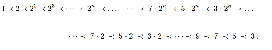
Figure 4: Sharkovskii’s ordering of natural numbers.
Logistic Map (Robert May, 1976)
\[x_n = a x_{n-1}(1 -x_{n-1})\]where $x_n$ population of species at $n$-th instance of time and $x_{n-1}$ is the population at $(n-1)$-th instant of time.
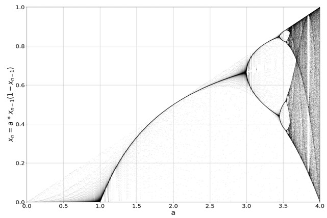
Figure 5. Bifurcation diagram of logistic map.
When $0<a<3$, we can see only period $1$. At $a=3$, we see the birth of period $2$.
Chaos in Movies
- Jurassic Park (1990)
- Sliding Doors (1998)
- Run Lola Run (1998)
- Tamil movie: 12B (2001)
Chaos in continuous time systems
Edward Lorenz an MIT meteorologist was trying to model the weather using a $12$- dimensional differential equation. A three dimensional version of the $12$-dimension equation is as follows: \(x^{'} = -10(x - y)\\ y^{'} = 28x - y - xz\\ z^{'} = xy - (\frac{8}{3})z\) This system of differential equation does not have an analytical solution because of the non-linearity. So Lorenz used a computer with a six digit precision to solve this computationally. He would run the simulation and printout the results. The computer worked with 6-digit precision, but the printout rounded variables off to a 3-digit number, so a value like 0.506127 printed as 0.506. This difference is tiny, and the consensus at the time would have been that it should have no practical effect. However, Lorenz discovered that small changes in initial conditions produced large changes in long-term outcome. Figure 6. shows an example for variation in prediction when the initial conditions are changed by a very small amount.
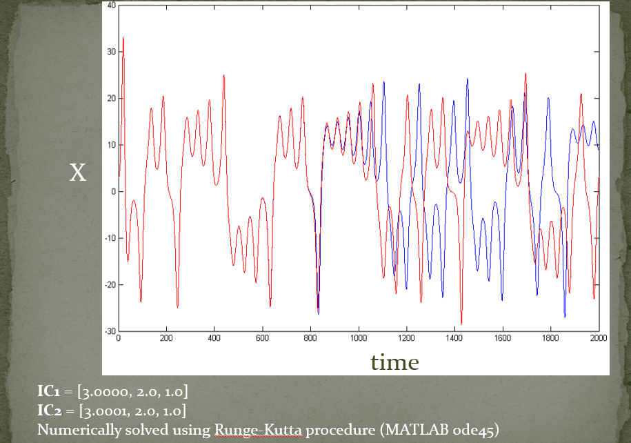
Figure 6: Solution for two different initial conditions ($IC$). $IC_1=[3.0000,2.0,1.0]$ and $IC_2=[3.0001,2.0,1.0]$.
Lorenz’s 1963 paper - Deterministic Nonperiodic Flow
“Two states differing by imperceptible amounts may eventually evolve into two considerably different states … If, then, there is any error whatever in observing the present state—and in any real system such errors seem inevitable—an acceptable prediction of an instantaneous state in the distant future may well be impossible….In view of the inevitable inaccuracy and incompleteness of weather observations, ***precise very-long-range forecasting would seem to be nonexistent.***”
The phase space of Lorenz weather prediction model is provided in Figure 7. The coordinates represents ($x(t), y(t), z(t)$).
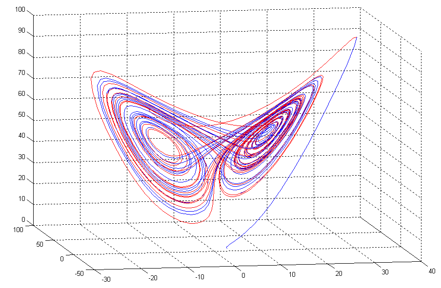
Figure 7: Phase space of Lorenz weather model.
This phase space provided in Figure 7 is also called strange attractor. There is a boundary for the phase space. The points inside the boundary goes to the strange attractor. The boundary of this strange attractor is a fractal. The points outside the boundary goes to infinity.
Leaky tap experiment.
Four grad students at U. Cal Santa Cruz -
Robert Shaw, J D Farmer, N Packard, James Crutchfield (Santa Cruz Chaos Cabal, 1984) looked at the leaky tap in the bathroom. They then decided to measure the time interval between two successive drops of the leaky tap. Then they found that this leaky tap experiment exhibited amazing chaotic patterns. This can be done by varying the flowrate of the tap. The details of this experiment are available in the book in Figure 8.

Figure 8: Chaotic dynamics in the leaky tap experiment. (Image Source: https://www.paperbackswap.com/Dripping-Faucet-Model-Chaotic-System/book/0942344057/)
Figure 9 shows how does the drop interval looks like.
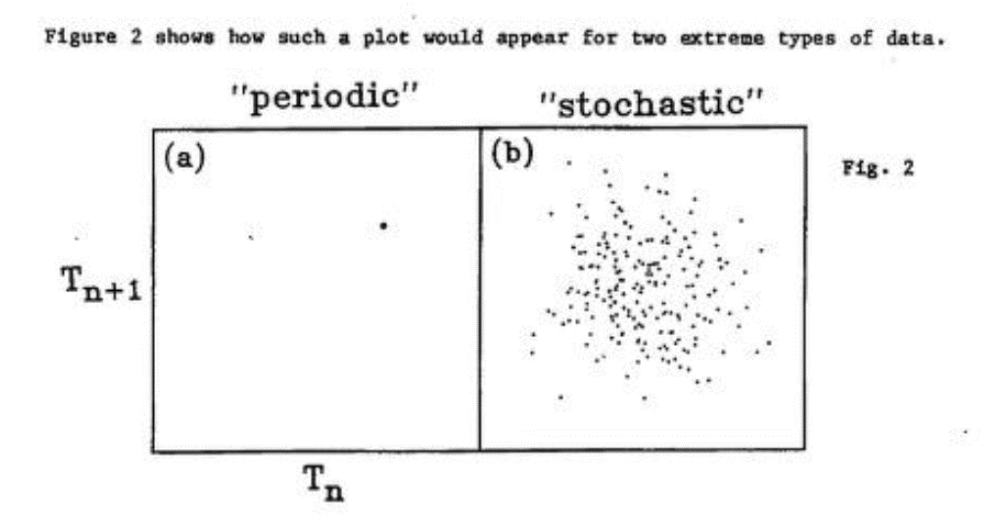
Figure 9 : Plot shows the drop interval of the leaky tap experiment. This figure is from the book The Dripping Faucet as a Model Chaotic System by Robert Shaw.
In Figure 9, (a) shows that the interval is regular. It shows a period-1 orbit. If it is period two, then there will be two points. But the graduate students found something very intersting. For a particular setting of the tap, we could have the drop interval of the leaky tap neither periodic and nor stochastic. This actually means there is chaos. Figure 10 represents this chaotic nature for a particular setting of leaky tap.
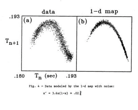
Figure 10: Chaotic dynamics in the leaky tap experiment. This figure is from the book The Dripping Faucet as a Model Chaotic System by Robert Shaw.
What can we understand from this experiment?
- Data driven model (not physics driven since it is too complicated)
- Continuous system discretized (Poincare section)
- Infinite dimensional system, but exhibits ‘low dimensional’ dynamics
- Chaos! – when flow rate is varied (periodic, semi-periodic or noisy periodic, irregular/non-periodic)
- Short term predictability, but long-term unpredictability
In the next class, mathematical understanding of chaos will be addressed.
Acknowledgement
Dr. Nithin Nagaraj would like to give credit to Dr. Kishor Bhat for the excel sheet chaos example and dedicate/thank the entire lecture (set of lectures) to late Prof. Prabhakar G Vaidya :)